Introduction

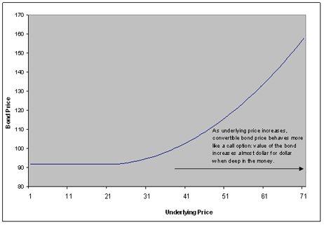
A convertible bond gives the holder the option to exchange (convert) the bond for a specified number of shares in the underlying company. The number of shares for which the bond can be exchanged is given by the conversion ratio, which is usually stated at bond issuance. While the investor holds the bond and does not exercise their option to convert, they will receive periodic payments at the stated coupon level. In essence, a convertible bond can be thought of as a regular bond with an embedded equity call option. Convertible bonds can also be issued with other embedded features such as time varying issuer calls and investor puts. As the underlying share price increases, the bond will behave more like an option.

» To download the latest trial version of FINCAD Analytics, contact a FINCAD Representative.

The main advantage to the issuer of a convertible bond is that the bond will usually be issued with a lower coupon rate than the equivalent non-convertible bond. This is because the holder of the convertible bond is compensated with the right to convert the bond into stock of the issuing company. If conversion does occur, dilution may also occur if new shares must be issued.

The valuation of a convertible bond is made more difficult due to the underlying characteristics. When pricing, one must consider the underlying bond and equity details. For example, the equity price, maturity, coupon, volatility and spread must all be considered. FINCAD currently has two methods for the pricing of convertible bonds: the first uses a trinomial tree and the second method, introduced in v10, uses a partial differential equation method, specifically the Crank-Nicolson finite-difference method.

FINCAD Methodology

Model

The model implemented is based on the paper by K. Tsiveriotis and C. Fernandes. The main idea behind this model is that a convertible bond consists of two components, an equity component and a debt component, and these components have different default risks. The equity component has no default risk since the issuer can always issue its own stock. Thus the equity component should be discounted at the risk-free rate. Coupon and principal payments, and any put provisions depend on the issuer's timely access to the required cash and thus introduce credit risk. Thus the debt component should be discounted at the risk-free rate plus a credit spread.

To split the convertible bond (CB) up into its components, a new hypothetical security is defined, called the "cash-only part of the convertible bond" (COCB). This hypothetical security is defined as follows: "The holder of a COCB is entitled to all cash flows, and no equity flows, that an optimally behaving holder of the corresponding convertible bond would receive." Since the convertible bond is a derivative of the underlying equity, the COCB must also be a derivative on the underlying equity, and the value of both should follow the Black-Scholes equation. This results in a system of two coupled Black-Scholes equations for the value of the convertible bond:

Equation 1

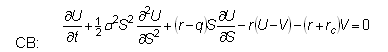
Equation 2

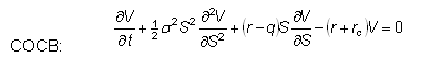
where U is the value of the convertible bond, V is the value of COCB, S is the underlying stock price, r is the risk free rate, q is the dividend yield, and rc is the credit spread.

The above system of coupled partial differential equations must be solved simultaneously. Looking at Equation 2, it appears at first that it is independent of Equation 1. However, the two equations are coupled due to the fact that this is a free boundary problem. The free boundary comes from the option to exercise at times other than maturity, and becomes an unknown in the problem that must be solved for at each time step. It is because of this common free boundary that Equations 1 and 2 are coupled and must therefore be solved simultaneously.

Currently FINCAD has two implementations of the above model for convertible bonds:

• Trinomial Tree
• Finite Difference Method

Trinomial Tree

This was the original FINCAD implementation for pricing convertibles. The stock price is modeled using a trinomial tree, and the value of the convertible bond is calculated at the final nodes based on any conversion options help at that time and then rolled back through the tree. This method is equivalent to a fully implicit finite difference scheme.

Finite Difference Method

In this implementation, the system of coupled partial differential is solved using a finite difference method, specifically the Crank-Nicholson scheme. This scheme is unconditionally stable and has better convergence properties than either the fully explicit or fully implicit schemes.

As part of the valuation process, a grid of time-steps is setup from the value date to the maturity date. The implementation also ensures that a time-step falls on every cash flow date, conversion dates, call and put dates and all discrete dividend dates.

For further details on the implementation, please refer to the "Convertible Bonds using PDE Methods" Math Reference.

Advantages of PDE

In v10, FINCAD made a decision to update the convertible bond functions using the PDE method. The key advantages that a user would see are in convergence to a solution and accuracy.

Convergence - The Crank-Nicolson method is unconditionally stable, having no relevant restriction on the number of time steps required to converge. The trinomial tree implementation can encounter convergence problems specifically when the underlying convertible bonds contains numerous features such as Bermudan calls/put at changing prices, changing conversion ratios and/or soft calls. The greater the number of additional features, the greater the number of timesteps required to ensure that all features are picked up by the trinomial tree.

Accuracy - the accuracy of the Crank-Nicolson method is better than our current tree implementation.

FINCAD - Features

FINCAD currently allows the user to model various different features that can be embedded within the convertible. Unless otherwise stated, both implementations can handle the feature listed below:

• Time varying conversion ratio
• Callable (European, Bermudan, or American)
• Putable (European, Bermudan, or American)
• Cap on Conversion Price
• Soft Calls
• Forced Conversion at Maturity
• Conversion rule regarding accrued interest and coupon
• Call rule regarding accrued interest and coupon
• Put rule regarding accrued interest and coupon
• Dilution Effect
• Cash Payments on Conversion
• Dividends - Although both models allow for discrete dividends and a yield, the PDE model allows the user to apply both a discrete dividend and a dividend yield, where the dividend yield would take affect after the date of the last discrete dividend given. This allows for discrete dividend payments to be used in the short term, while a dividend yield is used in the long term

Example

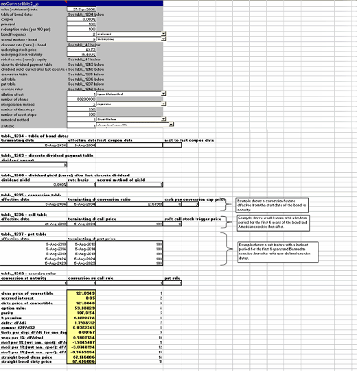
For an example of how a convertible bond can be set-up and priced using functions based on the PDE implementation, please see the spreadsheet below.

In this example, the details of the convertible bond issued by Henry Schein are entered in to the function aaConvertible2_p.

Disclaimer

Your use of the information in this article is at your own risk. The information in this article is provided on an "as is" basis and without any representation, obligation, or warranty from FINCAD of any kind, whether express or implied. We hope that such information will assist you, but it should not be used or relied upon as a substitute for your own independent research.

For more information or a customized demonstration of the software, contact a FINCAD Representative.