FINCAD has added curve building features (enhanced linear forward rates and quadratic forward rates) that further enable you to fine tune the pricing of your financial instruments. This article builds on a previously published article by FINCAD called "The Art and Science of Curve Building" released in the June 2004 issue of FINCAD News.
This is an older article written by FINCAD. For more information about FINCAD's modern curve-building approach, please click here.
To explore how you could use FINCAD Analytics Suite to build better curves, contact a FINCAD Representative and download the latest trial version of FINCAD Analytics.
At first glance, the mechanics of building a discount factor curve would appear to be a fairly mundane subject. At the very least, one would expect that it must be trivial, completely understood and there must be a market standard way of doing it. After all, a good interest rate curve is the most basic requirement for pricing and hedging interest rate derivatives. If the input curve is bad, no matter the model, it is guaranteed that the prices and hedging parameters it returns will be bad. As the saying goes: garbage in, garbage out. In fact, it turns out, that there is quite a bit of subtlety and flexibility in the curve building process. There is room for some (well thought-out) artistic license. Moreover, the subject is certainly not as well understood as it should be.
To illustrate, we will focus on the swap market. In this market, generally, the discount factor curve is built based on a combination of quoted money market and par swap rates. For the purposes of our discussion, the money market rates are not important. Our example is based on the following swap rate data:
| Term | Par Swap Rate |
| 2Y | 2.70% |
| 5Y | 3.60% |
| 10Y | 4.60% |
| 15Y | 4.80% |
| 20Y | 4.80% |
| 25Y | 4.75% |
The swaps pay annually and accrue 30/360. We chose these properties to eliminate the complications of having to consider accrual factors, even though real swaps are usually quarterly or semi-annual. This assumption means that a 4.6% swap pays a fixed coupon of 4.6% each year. For the sake of simplicity, we have further assumed that the swaps are spot settled.
Consistency is not enough
The process of building a discount factor curve from market quotes is known as bootstrapping. The basic requirement of the discount factor curve is that it be consistent with all input market rates. Consistent means that after we have built the curve, if we perform a round-trip calculation of, for example, the 10Y par swap rate, we indeed obtain 4.6% and similarly for all other rates.
It turns out that the consistency requirement is not enough. The bootstrapping process is (usually) an under-determined problem and we have a fair amount of flexibility in determining how the bootstrapping proceeds. We can take advantage of this flexibility to build better interest rate curves and we will use the structure of implied forward rates to guide our intuition on how to do it. Before we get ahead of ourselves, let's first understand some basic concepts.
Back to Basics
For a given date, a discount factor, also known as a zero coupon price, is the present value of one unit paid on that date. In our notation, Df1Y is the present value of one unit paid one year from today. A discount factor curve is a set of dates and discount factors. Given a discount factor curve, we can present value any future cash flow. A discount factor curve also contains other implied information, like the structure of forward rates. Given the one and two year discount factors, the one year implied forward rate, F, effective one year from today can be calculated from the formula, F=Df1y/Df2y-1.
Let's now look at the bootstrapping process and, to illustrate, we will focus on the 10Y par swap rate in our example. As we add (or bootstrap) this rate to the curve, it follows, by definition, that

Now the first 5 of these discount factors are known because we have already built a curve that includes the 5Y rate. Hence,

The right-hand side is known and, in this case, we have an under-determined system with one equation and 5 unknowns. At this point, in order to obtain a unique solution, constraints are added to the structure of the DfiY. Different constraints correspond to different bootstrapping methods.
Bootstrapping Method 1: Linear Swap Rates (LSR)
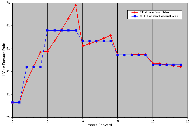
The first bootstrapping method we consider, Linear Swap Rates (LSR), assumes that the par swap rate at each intermediate coupon date lies on a straight line between the 5 and 10Y rates. In our example 6Y = 3.8%, 7Y = 4.0%, 8Y = 4.2% and the 9Y = 4.4%. With these constraints, we now solve for the discount factors. First, we solve for Df6Y,

Continue in the obvious way to calculate the 7, 8, 9 and 10-year discount factors. The results are shown in Figure 1a and labeled LSR. For a reference on the LSR method, see for example [3].
Bootstrapping Method 2: Constant Forward Rates (CFR)
The second method, Constant Forward Rates (CFR), constrains the problem by enforcing that all one year forward rates, effective at 5, 6, 7, 8 and 9 years, be equal. Let F be this rate. This implies Df6Y = Df5Y / (1 + F), Df7Y = Df5Y / (1 + F)2 and so on. In our example,
and it is straightforward to solve for F. The results are labeled CFR in Figure 1a.
This second bootstrapping method is fairly standard and we will go out on a limb and say it is the simplest "market standard" methodology.
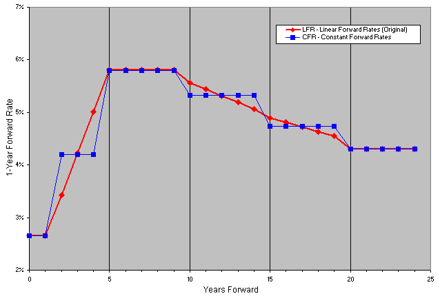
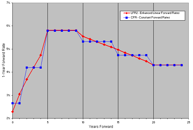
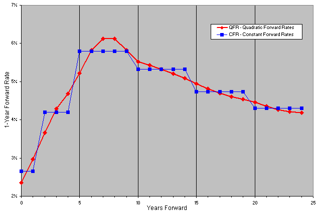
Figure 1: 1-year implied forward rates
Figure 1a
Figure 1b
Figure 1c
Figure 1d
Let's take a step back and analyze the two methods. In Figure 1a, we have plotted the one year implied forward rates. Let's focus on the LSR curve. At the short-end of the curve, the forward rate profile looks fairly good. After 7 years we see a disturbing pattern of "overshoots" where high rates are followed by much lower rates. It is a fact that the LSR methodology can often lead to this type of nasty behavior. On the other hand, the CFR curve does not have any of these overshoots. We see a pleasant looking step function, which in our example, happens to be humped. This shape was chosen in order to illustrate the features of the different methods offered in FINCAD Analytics Suite. If we only had the choice between these two methods, we would certainly choose to use the CFR. On the other hand, the resulting CFR curve is not completely satisfying. In this case, it seems reasonable to expect that the actual forward rates would be a little smoother (at the very least our artistic side says so).
Bootstrapping Method 3: Linear Forward Rates (LFR)
We now consider another bootstrapping methodology that we developed. We call it Linear Forward Rates (LFR). The first step in the LFR method is to calculate the CFR curve. The next step involves another bootstrapping pass to "smooth-out" the forward rates. During this step, as we splice each point to the curve, rather than looking for a constant forward rate F, we look for linear forward rates that lie on a line of the form F0 + K T, where K is the slope and F0 is chosen so as to best "fit" the current, previous and next forward rates. It turns out that the discount factors are best described in the following recursive way: Dfi+1 = Dfi /(1 + F0 + K Ti), where Ti is the time in years of the ith coupon period. In our example, Ti = 1 and if we again consider the 10Y point, it follows that

and we can solve for the slope K. When we are in a situation where the curve increases and then decreases (or vice versa), we do not modify the forward rates at these points. It turns out, that in this case, the best solution is to leave the forward rates in this region constant. We also leave the forward rates constant in the final segment (20 - 25 years), because we expect that the forward curve will become flat at the right-hand end. Likewise, we leave the forward rates constant in the first segment (0 - 1 years forward) if no short-term cash/futures rates are given. The results for our example are labeled LFR in Figure 1b. The CFR curve from Figure 1a is also shown to help with the visual comparison.
Bootstrapping Method 4: Enhanced Linear Forward Rates (LFR2)
The method is an enhancement of the original LFR algorithm, that produces smaller and fewer jumps in the forward curve. For example, a steeper slope is allowed in each segment if this eliminates a discontinuity with a neighboring segment. The match points are calculated using the results of the first pass, which as before uses the CFR method. It is not possible to completely eliminate all the jumps between the linear segments, and still preserve the round-trip on all the swap rates, but this enhanced algorithm is more aggressive at doing so than the original. The results for our example are labeled LFR2 in Figure 1c. There was a slight offset at 15 years using the LFR method (Figure 1b), that has been eliminated by using the LFR2 method (Figure 1c). Another change is that a slope is now allowed in the first segment (0 - 1 years forward) if no cash/futures rates are given. This enhanced LFR method is recommended over the original LFR method; the original method was retained for compatibility with previous versions of FINCAD XL
Bootstrapping Method 5: Quadratic Forward Rates (QFR)
This final method is similar to the LFR algorithm, except that instead of using straight-line segments for the forward curve, it uses parabolic segments. The end points of each segment match those of its neighbors. As before, a first pass is made using the CFR method, and the results are used to decide where the parabolic segments are going to match up. In the second pass, we look for forward rates that lie on a parabola of the form a + b T + c T2, so that the discount factors are Dfi+1 = Dfi /(1 + a + b Ti + c Ti2). The parameters a, b, and c for each segment are chosen to ensure that the curve is consistent with the given swap rates, and that the end points of each segment match those of its neighbors. The last segment is also parabolic, but is forced to be horizontal at its right-hand limit. The end result is a forward curve that is piecewise quadratic and continuous (no jumps). The results for our example are labeled QFR in Figure 1d.
Is Interpolation Good Enough?
Combining the QFR curve with some sort of interpolation method is recommended for most applications. But, what interpolation should we use?
Suppose, for example, we wanted to value a strip of three-month caps. Clearly, this derivative is extremely sensitive to the value of the underlying forward rates. We first choose to use the LFR2 curve in combination with one of the following four interpolation methods (for more details see for example [1], [2]).
1) Linear Discount Factors - discount factors between points are assumed to lie on a straight line
2) Linear Spot Rates - spot rates between points are assumed to lie on a straight line
3) Cubic Spline Discount Factors - The whole curve of discount factors lie on a "smooth" cubic spline (piecewise cubic, continuous and differentiable).
4) Exponential Discount Factors - discount factors between two points lie on an exponential curve of the form CeRT, where C and R are constants. This shape gives constant instantaneous forward rates between each pair of points.
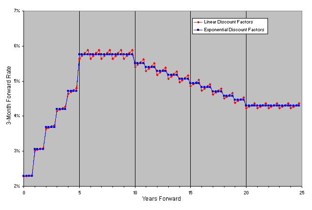
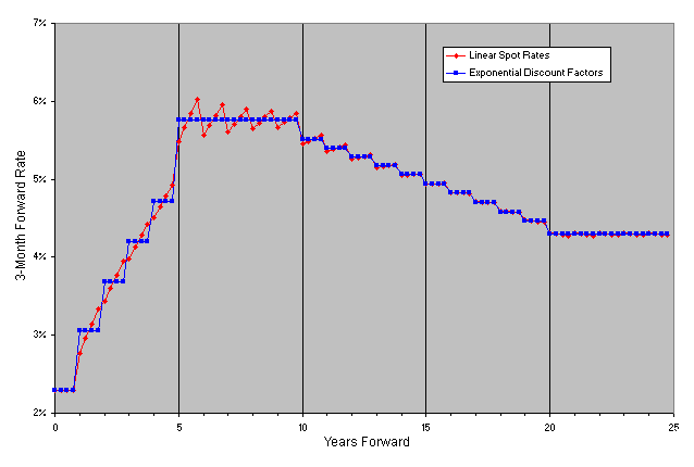
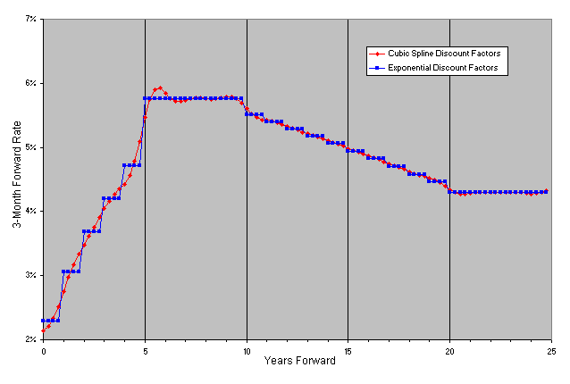
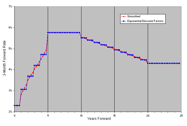
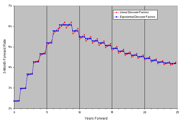
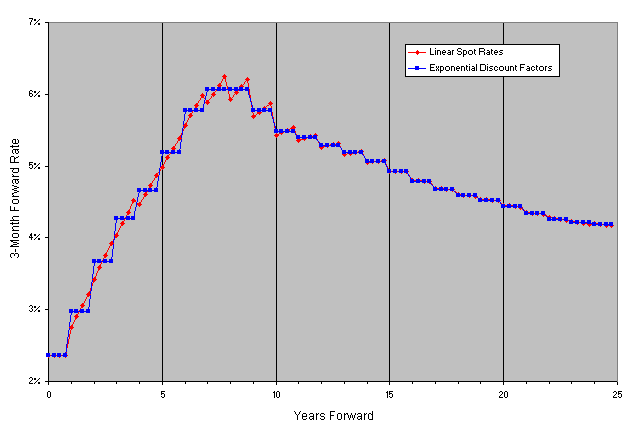
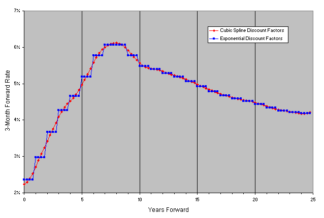
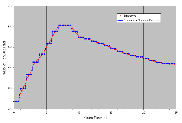
Figure 2: 3-month implied forward rates from the LFR2 curve
Figure 2a
Figure 2b
Figure 2c
Figure 2d
Looking at the 3-month forward rates in Figure 2a, we see that linear interpolation of discount factors has regions where a disturbing "saw-toothed" pattern appears where one would expect fairly constant forward rates. Not surprisingly, exponential interpolation of discount factors returns a "step-function" pattern of forward rates, since the instantaneous forward rates are constant in each year. In Figure 2b we see the same nasty "saw-toothed" pattern in the forward rates when we use linear interpolation of spot rates. The results obtained using the cubic spline look fairly good in Figure 2c, though there is a slightly disturbing "bulge" at around 5.5 years. It turns out that in some situations, when the underlying curve has jumps, the cubic spline, because it needs to be smooth and differentiable (while passing through all of the points), will bulge in regions leading to undesirable results like bad forward rates. There is also a very slight up-tick in the final forward rate (24.75 years forward), which is an artifact of the cubic spline method. The unfortunate conclusion is that none of these interpolation methods is perfect.
What is required is a method that combines the smoothness of cubic spline interpolation with the stability of exponential interpolation (in regions where the splines bulge). We know of no generic interpolation method that offers this. The good news is that we don't need a generic interpolation method, what we need is a method that is specific to discount factor curves. The method we have developed depends on applying a post-smoothing process to the curve. In this process, we enhance the discount factor curve (e.g. LFR2) by adding points at 3-month intervals (actually at any user desired frequency). We do this in such a way as to obtain smooth forward rates, in regions where the curve is smooth, while avoiding bulges in regions where the curve has "jumps". We stress that none of the original discount factors are altered and the enhanced curve remains consistent with the original input rates. The results of this curve are labeled "Smoothed" in Figure 2d. We would then use this enhanced discount factor curve as the basic input to our pricing function, and likely choose exponential interpolation for its interpolation method input (or any method, even linear interpolation, with this enhanced curve would be fine).
What about the situation where the original curve has no jumps? If we use the QFR curve in combination with one of the four interpolation methods described above, we obtain the results shown in Figure 3.
Figure 3: 3-month implied forward rates from the QFR curve
Figure 3a
Figure 3b
Figure 3c
Figure 3d
We see the same nasty "saw-toothed" pattern using linear interpolation of either discount factors (Figure 3a) or spot rates (Figure 3b) that we saw with the LFR2 curve. When we compare the results of the cubic spline interpolation (Figure 3c) with the post-smoothing function (Figure 3d), we no longer see any undesirable bulges in the splines. However, the slight up-tick in the final forward rate is still present in Figure 3c. Nonetheless, in this situation, we would choose the spline curve. We would therefore use the QFR curve as the basic input to our pricing function, and choose cubic spline interpolation for its interpolation method input.
The following table summarizes the recommended interpolation methods and post-smoothing requirements for the various bootstrapping methods:
| Bootstrapping Method | Post-smoothing Required? | Recommended Interpolation Method for Pricing Function |
| Linear Swap Rates (LSF) | Yes (although even post-smoothing cannot remove the original "overshoots" of Figure 1a) | Any |
| Constant Forward Rates (CFR) | No (it has no effect even if it is used) | Exponential (preserves constant forward rates) |
| Original Linear Forward Rates (LFR) | Yes | Any |
| Enhanced Linear Forward Rates (LFR2) | Yes | Any |
| Quadratic Forward Rates (QFR) | No | Cubic Spline |
The combination in the last row is recommended since it gives rise to the smoothest forward curve.
References
[1] H. Mathews, Numerical Methods for Computer Science, Engineering and Mathematics, 1987, Prentice Hall Inc,, Toronto.
[2] W.H. Press et al., Numerical Recipes in C, 1996, Cambridge University Press, New York
[3] Miron and Swannell, Pricing and Hedging Swaps, 1991, Euromoney Publications PLC, London
[4] U. Ron, "A Practical Guide to Swap Curve Construction", 2000, Bank of Canada Working Paper 2000-17 http://www.bankofcanada.ca/en/res/wp/2000/wp00-17.pdf
[5] P. Hagan & G. West (2004), "Interpolation methods for yield curve construction", submitted for publication.
Disclaimer
Your use of the information in this article is at your own risk. The information in this article is provided on an "as is" basis and without any representation, obligation, or warranty from FINCAD of any kind, whether express or implied. We hope that such information will assist you, but it should not be used or relied upon as a substitute for your own independent research.
For more information or a customized demonstration of the software, contact a FINCAD Representative.

