Overview

Synthetic collateralized debt obligations (CDOs) are credit derivatives that are "synthesized" through credit derivatives, such as credit default swaps (CDSs), on a pool of reference entities. Such reference entities can be bonds, loans or simply names of companies or countries. Most synthetic CDOs in the market do not have a so-called cash flow waterfall structure. They can be customized so that the payment structure of a tranche doesn’t depend on the payment structures of other tranches. Such CDOs are thus sometimes called single tranche CDOs. Single tranche CDOs have been developing rapidly for the last few years and are the most popular synthetic CDOs currently in the market. The most popular single tranche CDOs are exchange traded standardized tranches. The reference credit pools of such CDOs are CDS indices, such as CDX and ITRAXX series. Other (non-standard) single tranche CDOs are often called bespoke tranches.

To download the latest trial version of FINCAD Analytics Suite, contact a FINCAD Representative.

A common structure of CDOs involves slicing the credit risk of the reference pool into a few different risk levels. The level with a higher credit risk supports the levels with lower credit risks. The risk range of two adjacent risk levels is called a tranche. The lower bound of the risk level of a tranche is often referred to as an attachment point and the upper bound a detachment point. For example, a 5-10% tranche has an attachment point of 5% and a detachment point of 10%. When the accumulated loss of the reference pool is no more than 5% of the total initial notional of the pool, the tranche will not be affected. However, when the loss has exceeded 5%, any further loss will be deducted from the tranche’s notional until the detachment point, 10%, is reached.

The most commonly used credit derivatives in synthetic CDOs are credit default swaps (CDSs on CDO tranches) and tranche-linked notes (CDO notes). They can be viewed as extensions of the corresponding single entity credit default swaps and credit-linked notes. Like a single-entity CDS, a CDS on a CDO tranche has a payoff leg and a premium leg. The buyer of a CDS on a tranche will be compensated by the seller for any loss to the tranche and in return he/she pays periodic premium to the seller. As the loss to the tranche increases, the premium notional of the tranche decreases and hence the premium payment decreases. In the case of a CDO note the buyer of a CDO note pays upfront a certain amount, called the note’s principal, and receives periodic coupon payments and its principal at maturity if the tranche that the note is linked to doesn’t suffer a loss. However, when the accumulated loss of the reference entities eats into the tranche, the note’s principal will be reduced by the lost amount and thus the future coupon and principal payment will be reduced. The main differences between a CDO credit derivative and a single-entity credit derivative are twofold: (1) a CDO derivative has a variable notional whereas a single entity credit derivative has a constant notional; (2) a CDO derivative has a protection layer (except for an equity tranche derivative) whereas a single-entity derivative does not.

Valuation

Monte Carlo simulation has been the most popular method for CDO valuation. It is flexible and relatively simple for implementation. The disadvantage is that Monte Carlo simulation can be resource intensive for large CDOs. In recent years non-Monte Carlo methods, also known as quasi-analytic or semi-analytic methods, have become more and more popular. They are more efficient than Monte Carlo simulation for certain types of synthetic CDOs, particularly, standardized tranches, when a one-factor copula model is used for modeling credit correlation of reference entities.

FINCAD Analytics Suite provides both Monte Carlo simulation-based and quasi-analytic method-based tools to value synthetic CDOs.

1. Valuing CDOs with Monte Carlo Simulation

Valuing a synthetic CDO contract using Monte Carlo simulation is straightforward. First, generate default scenarios of the reference entities based on the Gaussian copula model (Li model) or the multi-step credit index model (Hull-White model). Then, calculate the loss amount to the tranches for each scenario. Next calculate the present values of the default leg and the premium legs for a CDS, or coupons and the principal for a CDO note. At last calculate the average present values.

The FINCAD Analytics Suite Monte Carlo simulation-based tools can be used to value

• CDS on CDO tranches, including both standard tranches and bespoke tranches.
• Fixed rate CDO notes, notes that are linked to CDO tranches.
• CDOs with counterparty default risk.
• First loss CDSs.

2. Valuing CDOs with FFT (a quasi-analytic method)

In the valuation of a CDO, the key is to calculate the loss distribution of the reference pool. Let L(T) be the total loss, up to time T , of the entities in a reference credit pool. To calculate the distribution of L(T) we only need to determine its characteristic function

f (t) = E exp(−tL(T )).

For this a natural choice is the FFT (fast Fourier transform). When the characteristic function has been determined, the reverse FFT can be used to back out the loss distribution.

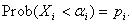
The determining factors of the above characteristic function are the default probabilities of the reference credits and their default correlations. The default probabilities can be obtained from other sources, such as credit default swap spreads and bond yields. Hence the key to the valuation of a CDO is the modeling of default correlation of the reference credits. The current market standard model on default correlation is the Gaussian (normal) copula model. Under this model the credit index (roughly, the asset return) of a firm has the following form

where are independent Gaussian random variables with mean 0 and standard deviation 1 (N(0, 1)) and α_i, called the factor loading of entity i , is a constant between -1 and 1. A higher value of X_i represents a higher credit quality of the entity. Given a default probability p_i of the entity one can then find a threshold value of α_i of X_i such that

Since X_i is an N(0,1) variable, , where Φ is the cumulative distribution function of an N(0,1) variable. With the Gaussian copula model we can determine the credit correlation easily by simply using the joint probability

Pr ob(X_i α_i , X_j α_j ) =Φ₂(ρ_{i, j} ,α_i ,α _j )

where is the correlation of X_i and X_j and Φ₂ is the cumulative standard bivariate normal distribution function.

A special case of the Gaussian copula model is the one for which all factor loadings are equal. For this case each pair of the reference entities has the same correlation, ρ, and the factor loading is the square root of the correlation:

Tools for valuing CDSs using FFT on synthetic CDO tranches based on the one -factor Gaussian copula model are available in FINCAD Analytics Suite. These tools can handle both variable factor loadings and a constant factor loading (a single correlation). For the case of a single correlation they can handle both tranche correlations (also known as compound or implied correlations) and base correlations. In addition to fair value calculation, these tools calculate a variety of sensitivities. Their outputs include:

• Fair values of tranche CDSs and values of payoff and premium legs
• Expected premium cash flows
• Par CDS spreads
• DVOX – sensitivity of credit spreads
• Deltas on individual entity credit spreads
• Rho of recovery rates
• Rho of correlation or factor loadings

For CDO portfolios these tools are particularly friendly: they can value multiple tranches simultaneously.

3. Default Correlation Calibration

Under a one-factor copula model with a constant factor loading the default correlation of the credits in a reference pool is captured by a single asset correlation. A natural question to ask is: given the premium spread of a CDS on a CDO tranche can one find an asset correlation under which par spread of the tranche is the given spread, and if such an correlation exists, is it unique? Such a correlation is also called a tranche or compound correlation. Research shows that, under the Gaussian copula model, for an equity tranche the answer is a "yes" for both questions, but for a mezzanine tranche only the existence question has a "yes" answer. Typically, for a mezzanine tranche there are two distinct correlations that give the same par spread. Such a lack of uniqueness makes such an implied correlation difficult to interpret and even more difficult to use in CDO hedging.

Due to this uniqueness problem many CDO users have abandoned the use of tranche correlation and moved to another type of correlation, the so-called base correlation, proposed by L. McGinty of J P Morgan. A base correlation is the extension of the compound correlation of an equity tranche. For a mezzanine tranche the tranche that has an attachment of 0 and the same detachment point of the given tranche is called the base tranche of the mezzanine tranche. The implied correlation that applies to the base tranche is called the base correlation of the mezzanine tranche. As mentioned above base correlations are uniquely defined.

Since premium spread quotes are for regular tranches only, the implied base correlation of a tranche cannot be obtained directly. To calculate the base correlation a so-called bootstrapping method must be used. For details on base correlation bootstrapping the reader is referred to the FINCAD Analytics Suite math document Synthetic CDO Valuation Using Quasi-Analytic Methods.

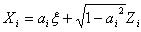
Due to imperfect modeling of correlation, the implied base correlation of a CDO is not a constant, in stead, it varies with tranches. Typically, a base correlation curve is skewed. An example of a base correlation curve is given in the figure below.

FINCAD Analytics Suite has tools to calculate implied base correlations. These tools can handle both standardized and bespoke CDOs.

An example of a single tranche CDO

Consider a synthetic CDO with a reference credit pool of 125 names and a time to maturity of 5 years. It has five tranches: 0-3%, 3-7%, 7-10%, 10-15% and 15-30%. Each of the names has the same notional of 1000000, the same recovery rate of 40% and also the same flat CDS spread of 0.5% at the 0.5, 1, 2, 3, 5, 7 and 10 year time points. The premium payment frequency of all the tranches are quarterly and the accrual method is actual/365. The running spreads of the tranches are 500, 100, 30, 20 and 10 basis points, and the base correlations are 7%, 22%, 30%, 40% and 63%, respectively. Given a flat default-free rate of 5%, the CDSs on these tranches, with a protection-buy position for each tranche, have the fair values and break-even spreads shown in the following table

output type \ tranche	0-3%	3-7%	7-10%	10-15%	15-30%
fair value	1679551.58	10920.54	-3506.99	-9118.00	-31964.91
payoff value	2206052.20	231535.42	46645.26	46667.77	51841.09
premium value	-526500.62	-220614.88	-50152.24	-55785.77	-83806.00
break-even spread (bp)	2095	105	28	17	6

If the equity tranche has an upfront fee of 40%, then the break-even spread of the tranche will be 671 basis points, instead of 2095 bps.

The above results are produced with the FINCAD Analytics Suite CDO valuation function aaCDO_ST_DS_std_p.

Disclaimer

Your use of the information in this article is at your own risk. The information in this article is provided on an "as is" basis and without any representation, obligation, or warranty from FINCAD of any kind, whether express or implied. We hope that such information will assist you, but it should not be used or relied upon as a substitute for your own independent research.

For more information or a customized demonstration of the software, contact a FINCAD Representative.