

FINCAD Analytics Suite for Excel and FINCAD Analytics Suite for Developers expand FINCAD's ability to calculate various counterparty credit exposure metrics by adding credit exposure functions for a portfolio of interest rate swaps.
Contact a FINCAD Representative for a free evaluation of FINCAD Analytics.
Overview
Counterparty credit exposure is a measure of the amount that would be lost in the event that a counterparty to a financial contract defaults. Only contracts that are privately negotiated between counterparties, i.e. over-the-counter (OTC) derivatives, are subject to counterparty credit risk. Contracts that are traded on an exchange are not affected by counterparty risk, because the exchange guarantees the cash flows promised by the derivative to the counterparties [2].
In a plain vanilla interest rate swap, the counterparties agree to exchange a payment based on a fixed rate for a payment based on a floating rate. If the floating rate is above the fixed rate, then the floating rate payer will make a payment to the floating rate receiver based on the difference between the two rates. If the floating rate payer defaults, this will lead to a credit loss for the floating rate receiver. Assuming that no recovery is possible, the total loss will be the present value of the net interest payments remaining. This is known as the replacement cost of the swap, and is a commonly used measure of credit loss.
If a contract has positive value for the counterparty that does not default, then the replacement cost will be the market value of the contract, since this is what they would have to pay to purchase a replacement contract on the market. However if the contract has negative value for the counterparty that does not default, this counterparty does not get to walk away from the contract in the event that their counterparty defaults. For this reason, the replacement cost is the greater of the fair market value of the contract and zero. This is known as current credit exposure. While this is a useful and commonly used metric of credit exposure, it only provides a snapshot of the exposure at a single point in time. The value of derivative contracts can fluctuate significantly over time, therefore it is also very useful to consider the credit exposure at future times. This is known as potential credit exposure. Only the current exposure is known with certainty, while the future potential exposure is uncertain.
Potential credit exposure is an estimate of the replacement cost of the contract at various times in the future. Commonly, a time horizon of six months to a year is used, with contract values calculated at various times over the time horizon. In FINCAD Analytics Suite 2009, a 1-factor short rate model implemented on a trinomial tree is used in order to estimate the range of possible future values for a portfolio of interest rate swaps, each of which can be non-amortizing or amortizing. The swaps are with the same counterparty, and netting agreements can be taken into account (see below). If there is only one swap with the counterparty, then the same functionality can be used by setting up a portfolio containing just a single swap. Based on the trinomial interest rate tree, a probability distribution is calculated at future time points, from which the expected level of credit exposure that is unlikely to be exceeded at a given confidence level is calculated. For example, we can calculate the distribution of portfolio values one year from present and take the 95th percentile of this distribution.
Credit Exposure Metrics
Netting Agreements
The above definition of Potential Future Exposure assumes that no netting agreements are in place. Netting agreements are risk mitigants built into the derivative contract, where in the event of default the marked-to-market values of all the derivative positions between the two parties that have netting agreements in place are aggregated, i.e., positions with positive value can be used to offset positions with negative value. Therefore only the net positive value represents the credit exposure at the time of default. Assuming that netting agreements are in place, the Potential Future Exposure is

Having netting agreements in place reduces the overall credit exposure for the portfolio. The FINCAD functions aaCE_SwapPort_dgen, aaCE_SwapPort_dgen_tbl, and aaCE_SwapPort_dgen_dist all assume that all swaps in the portfolio are covered by netting agreements. In cases where there are no netting agreements, portfolio credit exposure can be calculated by summing the exposures of the individual swaps in the portfolio.
Peak Exposure and Maximum Peak Exposure
The Peak Exposure (PE) is the maximum amount of exposure expected to occur on a future date at a given level of confidence. For example, the 95%PE is the level of potential exposure that will not be exceeded with 95% confidence. The curve PE(t) is the peak exposure profile up to the final maturity of the portfolio. The peak exposure is defined by confidence level for which we want to calculate the peak exposure.
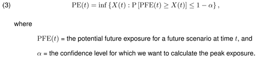
The maximum value of PE(t) over any given time horizon is referred to as the Maximum Peak Exposure (MPE). This can be calculated using the FINCAD function aaCE_SwapPort_dgen, which also returns the date at which the Maximum Peak Exposure occurs.
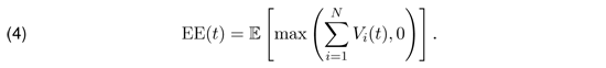
Expected Exposure
The Expected Exposure (EE) is the average of the distribution of exposures at any particular future date before the longest maturity in the portfolio. The expected exposure at time t is
Expected Positive Exposure
The Expected Positive Exposure (EPE) is the weighted average over time of the expected exposure, where the weights are the proportion that an individual expected exposure represents of the entire exposure horizon time interval [1]. The EPE can be calculated as
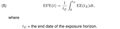
The integral is performed over the entire exposure horizon time interval starting from today (time 0) to the exposure horizon end date. In practice, this integral is approximated by a sum over all the tree time step dates up the exposure horizon end date.
Effective Expected Exposure
Effective Expected Exposure (EEE) is the maximum expected exposure which occurs over the exposure horizon time interval. The EEE can be calculated as
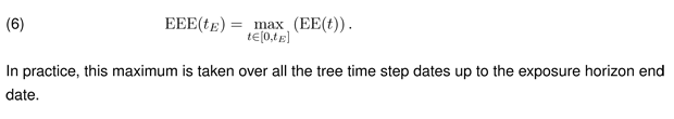
In practice, this maximum is taken over all the tree time step dates up to the exposure horizon end date.
Effective Expected Positive Exposure
Effective Expected Positive Exposure (EEPE) is the weighted average over time of effective expected exposure. The weights are the proportion that an individual exposure represents of the entire exposure horizon time interval. The EEPE can be calculated as

In practice, this integral is approximated by a sum over all the tree time step dates up the exposure horizon end date.
Example: Swap Portfolio Peak Exposure Profile
In this example we calculate several credit exposure metrics for a portfolio of swaps. Suppose that counterparty A has entered the following interest rate swap contracts with counterparty B:
| Swap #1 | Swap #2 | Swap #3 | |
| Effective Date | 15-Oct-2006 | 15-Jun-2004 | 10-Aug-2007 |
| Terminating Date | 15-Oct-2011 | 15-Jun-2014 | 10-Aug-2012 |
| Frequency | Semi-Annual | Semi-Annual | Semi-Annual |
| Fixed Coupon | 5% | 5% | 5% |
| Structure | Pay Floating | Pay Floating | Pay Floating |
| Amortizing | Anually | No | No |
Using the FINCAD function aaCE_SwapPort_dgen_tbl, we can output various exposure metrics, and graph the peak exposure profile over the remaining life of the portfolio.
As we can see in Figure 4, the Maximum Peak Exposure is projected to occur around May 2010 with a 95% Peak Exposure of about $252,000. The Peak Exposure declines after this date because the swaps are getting closer to maturity and there are fewer remaining cash flows.
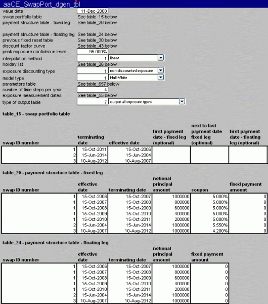
Figure 1: Screenshot of inputs to aaCE_SwapPort_dgen_tbl.
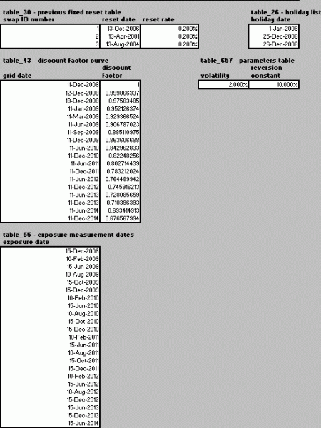
Figure 2: Screenshot of inputs to aaCE_SwapPort_dgen_tbl.
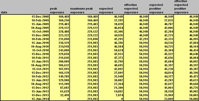
Figure 3: Exposure metrics output from aaCE_SwapPort_dgen_tbl.
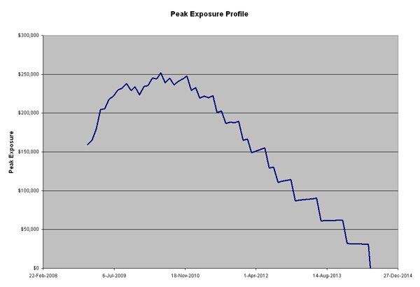
Figure 4: Graph of peak exposure profile output from aaCE_SwapPort_dgen_tbl.
Summary
FINCAD Analytics Suite 2009 provides functions to calculate various credit exposure metrics for a portfolio of swaps. aaCE_SwapPort_dgen can be used to calculate exposures over a given time horizon, while aaCE_SwapPort_dgen_tbl can be used to calculate exposure profiles given a set of future exposure measurement dates. There is also a utility function, aaCE_SwapPort_dgen_dist, that can be used to calculate the cumulative probability distribution at a given time in the future.
Reference
[1] Zhu, Steven H. and Pykhtin, Michael (2006), Measuring Counterparty Credit Risk for Trading Products under Basel II, Risk Books.
[2] Zhu, Steven H. and Pykhtin, Michael (July/August 2007), A guide to modeling counterparty credit risk, GARP Risk Review.
For more information or a customized demonstration of the software, contact a FINCAD Representative.